Lecture 6 - Ch 8b - Confidence Interval for the Mean with *Unknown* Std Dev

The Central Limit Theorem tells us that xbar (the mean of a sample) is normally distributed around the population mean with std dev of sigma/sqrt(n).

Equivalently, we can say that the z-score (xbar-mu)/(sigma/sqrt(n)) is normally distributed around 0 with std dev of 1.

In the case where we don't know the standard deviation of the mean, we can only look at the distribution of the variable t = (xbar-mu)/(s/sqrt(n)), where s is the std dev of the sample.

In the early 1900s, a statistician for Guinness Brewery (now that's a job I'd like to have!) developed a formula for the t distribution as a function of n. Actually, it's usually expressed as a function of (n-1) which is called the "degrees of freedom" in the sample.

The actual function for t is incredibly complex. It looks like this: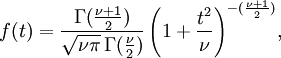
Please, do not try to remember that!

What you do need to know is that just like the binomial, poisson and normal distributions, math majors seeking something productive to do have spent countless hours calculating the values for the t-distribution and putting them in tables.

The way the t-table works is almost the opposite of the way the normal distribution table works. The normal distribution table assumes you know a z-score and the table tells you the area under the curve corresponding to that z-score (either from the mean to the z-score in table e.11 or from -infinity to the z-score in table e.2).

The t-distribution table assumes you know the area under the curve and the degrees of freedom (n-1) and the table tells you the corresponding "t-score", which is called the Critical Value.

The shape of the t-distribution is similar to the normal distribution except that it has fatter tails at low values of n. As n gets larger, the t-distribution is almost identical to the normal distribution. In class, we said that they are essentially identical for n>=30. In the book, it gives a value of 120 for n for the two distributions to be considered identical.

To graphically demonstrate how the t-distribution converges on the normal distribution as n increases, we watched an online java applet demonstration that allows us to manually vary n and watch how the two distributions become more and more similar as n increases.